
This post is about two popular-mathematics books the I recently read:
MY BRAIN IS OPEN: The Mathematical Journeys of Paul Erdős / Bruce Schechter
On one occasion, Erdős met a mathematician and asked him where he was from. “Vancouver,” the mathematician replied. “Oh, then you must know my good friend Elliot Mendelson”, Erdős said. The reply was “I AM your good friend Elliot Mendelson.”
Several years ago I read another biography of Erdős by Paul Hoffman, which was nice, though focused mainly on Erdős’s eccentricities. I think that Schechter’s biography would appeal more to mathematicians, since it consists of a lower dose of eccentricities and of a higher dose of details about the mathematical world. For example, it was very interesting to read about how a Hungarian mathematics journal for high school students helped in the nurturing of many great mathematicians, and about the events that led to the elementary proof for the prime number theorem by Selberg and Erdős. I definitely recommend this book.
For those who are looking for an even lower dose of eccentricities and more details about the mathematical world, I recommend the piece “In and Out of Hungary, Paul Erdös, His Friends, and Times” by László Babai. It can be found in volume 2 of Combinatorics, Paul Erdös is eighty, and it contains many details about the Hungarian mathematical world (and about 20-th century Hungarian history in general).


On one occasion, Erdős met a mathematician and asked him where he was from. “Vancouver,” the mathematician replied. “Oh, then you must know my good friend Elliot Mendelson”, Erdős said. The reply was “I AM your good friend Elliot Mendelson.”


Mathematical Cranks / Underwood Dudley
Represent heaven, the home of God, as a vector space of infinite dimension over some field
known to god but unknown to us, in which the activities of God are quantifiable. Lengths will be measured (Revelation chapter 21 verse 15) in the usual way, as the square roots of the inner self-products of vectors (assuming heaven to be euclidean).
 for the Erdős distinct distances problem (where
  denotes the number of distinct distances that are determined by pairs of points from
  , and
, and  ). The best known upper bound is
  , which leaves a gap of
  . The common belief is that
  , and thus, that there should exist a way to strengthen the analysis of the lower bound.
 distinct distances, for which the Elekes-Sharir framework can only yield a bound of
  . Such configurations imply that to improve the Guth-Katz lower bound while by relying on the Elekes-Sharir framework, one either has to make a drastic change in the framework, or to separately handle the family of “problematic” point configurations.

 .
. points and let
  be a set of
  planes, both in
  such that all the points of
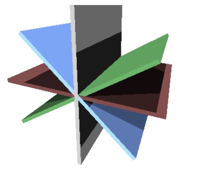
 , which makes the problem not interesting. There exist several definitions of non-degenerate point-plane configurations, which make the problem of bounding the number of incidences more challenging (e.g., see
  (they study the dual setting where no three points are collinear, though it is equivalent to our setting). A more general case is studied in a yet unpublished manuscript by
  planes (and
  .
. .
. ). Thus, the Kővári–Sós–Turán theorem implies

 , we avoided the main difficulty in applying the technique, which arises only in dimensions
  – bounding the number of incidences on the partitioning itself (i.e., on the zero set of the partitioning polynomial). In the plane, the partitioning is a one-dimensional curve, which is relatively simple to handle. Already when dealing with point-curve incidences in
  -dimensional patch, for otherwise no further partitioning would take place.
 of the ambient space as a constant, and ignore the dependence on
 ![f\in{\mathbb R}[x_1,\ldots,x_d]](https://s0.wp.com/latex.php?latex=f%5Cin%7B%5Cmathbb+R%7D%5Bx_1%2C%5Cldots%2Cx_d%5D++&bg=ffffff&fg=000000&s=1&c=20201002) of degree
of degree  , a parameter
  , and a finite point set
 ![g\in{\mathbb R}[x_1,\ldots,x_d]](https://s0.wp.com/latex.php?latex=g%5Cin%7B%5Cmathbb+R%7D%5Bx_1%2C%5Cldots%2Cx_d%5D++&bg=ffffff&fg=000000&s=1&c=20201002) of degree at most
of degree at most  , co-prime with
  , which partitions
  and
and  , for
, for  , so that each
  , for
, for  , lies in a distinct component of
  , and
, and  .
.